Here's something encrypted, password is required to continue reading.
Read more
n## 重要的日子
7/1:♥️糖醋羊排CP成立!!♥️
爱心屋签到: aixinwu.sjtu.edu.cn/products/asw-store
每日二GRISSO💊, 米诺地尔
Starting from 10/9:
| Time | Monday | Tuesday | Wednesday | Thursday | Friday | Saturday | Sunday |
|---|---|---|---|---|---|---|---|
| 08:00 | |||||||
| 09:00 | |||||||
| 10:00 | 攀爬机器人组会 | ||||||
| 11:00 | |||||||
| 12:00 | |||||||
| 13:00 | |||||||
| 14:00 | |||||||
| 15:00 | |||||||
| 16:00 | |||||||
| 17:00 | |||||||
| 18:00 | |||||||
| 19:00 | |||||||
| 20:00 | |||||||
| 21:00 | |||||||
| 22:00 | |||||||
| Credits: No need |

Bayes’ Theorem | Bayesian Inference
贝叶斯公式(Bayes’ Theorem)是概率论中的基本定理,描述了如何根据新证据更新对事件概率的信念。它是贝叶斯统计学、机器学习、人工智能等领域的理论基础,提供了一种系统化的方法来处理不确定性和进行推理。
$$P(A|B) = \frac{P(B|A) \times P(A)}{P(B)}$$
$$P(\theta|D) = \frac{P(D|\theta) \times P(\theta)}{P(D)}$$
或写成:
$$\text{后验概率} = \frac{\text{似然} \times \text{先验}}{\text{证据}}$$
| 符号 | 名称 | 含义 |
|---|---|---|
| $P(\theta|D)$ | 后验概率 | 看到数据 $D$ 后,参数 $\theta$ 的概率 |
| $P(D|\theta)$ | 似然 | 给定参数 $\theta$,观测到数据 $D$ 的概率 |
| $P(\theta)$ | 先验概率 | 看到数据前,对参数 $\theta$ 的初始信念 |
| $P(D)$ | 边缘似然/证据 | 数据 $D$ 出现的总概率(归一化常数) |
$$P(D) = \int P(D|\theta)P(\theta)d\theta$$
或离散情况:
$$P(D) = \sum_{\theta} P(D|\theta)P(\theta)$$
贝叶斯公式回答:**”看到证据后,我应该如何更新我的信念?”**
$$\text{新信念} = \frac{\text{旧信念} \times \text{证据支持度}}{\text{归一化}}$$
核心思想:
场景:
问:你真的患病的概率是多少?
解答:
设:
已知:
计算边缘似然:
$$P(B) = P(B|A)P(A) + P(B|\neg A)P(\neg A)$$
$$= 0.95 \times 0.01 + 0.05 \times 0.99 = 0.059$$
应用贝叶斯公式:
$$P(A|B) = \frac{P(B|A) \times P(A)}{P(B)} = \frac{0.95 \times 0.01}{0.059} \approx 0.16$$
结论:即使测试阳性,患病概率只有 **16%**!
反直觉原因:先验概率很低(1%),大部分阳性结果来自假阳性。
场景:
问:含”中奖”的邮件是垃圾邮件的概率?
解答:
设:
已知:
计算:
$$P(W) = 0.8 \times 0.3 + 0.05 \times 0.7 = 0.275$$
$$P(S|W) = \frac{0.8 \times 0.3}{0.275} \approx 0.87$$
结论:含”中奖”的邮件有 87% 概率是垃圾邮件。
场景:训练一个分类模型
目标:找到最优参数 $\theta$
$$P(\theta|D) = \frac{P(D|\theta) \times P(\theta)}{P(D)}$$
最大后验估计(MAP):
$$\theta_{MAP} = \arg\max_{\theta} P(\theta|D) = \arg\max_{\theta} P(D|\theta)P(\theta)$$
根据领域知识或假设选择先验分布:
$$P(\theta)$$
常见先验:
观测数据 $D = {x_1, x_2, \ldots, x_N}$
根据模型计算数据的似然:
$$P(D|\theta) = \prod_{i=1}^{N} P(x_i|\theta)$$
计算后验分布:
$$P(\theta|D) = \frac{P(D|\theta)P(\theta)}{P(D)}$$
| 方面 | 贝叶斯学派 | 频率学派 |
|---|---|---|
| 参数性质 | 随机变量(有分布) | 固定未知值 |
| 概率含义 | 信念程度 | 长期频率 |
| 推断方法 | 后验分布 | 点估计 + 置信区间 |
| 先验知识 | 必须指定先验 | 不使用先验 |
| 不确定性 | 参数的概率分布 | 估计的抽样分布 |
| 小样本 | 可利用先验 | 可能不稳定 |
问题:抛硬币 10 次,8 次正面,估计正面概率 $\theta$
频率学派:
$$\hat{\theta}_{MLE} = \frac{8}{10} = 0.8$$
贝叶斯学派(假设先验 $\theta \sim \text{Beta}(2,2)$):
$$P(\theta|D) = \text{Beta}(2+8, 2+2) = \text{Beta}(10, 4)$$
后验均值:
$$\mathbb{E}[\theta|D] = \frac{10}{10+4} \approx 0.71$$
差异:贝叶斯方法考虑了先验信念(硬币应该接近公平),结果更保守。
$$P(y|x_1, \ldots, x_n) = \frac{P(y) \prod_{i=1}^{n} P(x_i|y)}{P(x_1, \ldots, x_n)}$$
应用:文本分类、垃圾邮件过滤
$$P(w|D) = \frac{P(D|w)P(w)}{P(D)}$$
优势:提供预测的不确定性
对网络权重建模为分布而非点估计:
$$P(w|D) \propto P(D|w)P(w)$$
应用:不确定性量化、主动学习
当后验 $P(\theta|D)$ 难以计算时,用简单分布 $q(\theta)$ 近似:
$$\min_q D_{KL}(q(\theta)||P(\theta|D))$$
应用:VAE、主题模型(LDA)
通过采样近似后验分布:
$$\theta^{(t+1)} \sim P(\theta|D)$$
应用:贝叶斯深度学习、概率编程
目的:表达”无知”
例子:
定义:后验与先验同分布族
例子:
| 似然 | 共轭先验 | 后验 |
|---|---|---|
| 伯努利 | Beta | Beta |
| 正态(已知方差) | 正态 | 正态 |
| 泊松 | Gamma | Gamma |
| 多项式 | Dirichlet | Dirichlet |
优势:后验有闭式解,计算简单
目的:防止过拟合
例子:
从数据中估计先验的超参数:
$$\hat{\alpha} = \arg\max_{\alpha} P(D|\alpha)$$
回答:
回答:
回答:
回答:可以!这是贝叶斯方法的优势。
顺序更新:
$$P(\theta|D_1, D_2) = \frac{P(D_2|\theta)P(\theta|D_1)}{P(D_2|D_1)}$$
前一次的后验成为下一次的先验:
1 | 先验 → [数据1] → 后验1 → [数据2] → 后验2 → ... |
1 | # 弱信息先验(数据主导) |
1 | # 先验预测检查 |
1 | # 后验预测检查 |
1 | # 避免数值下溢 |
1 | import torch |
Variational Inference | Evidence Lower Bound | VAE Paper
ELBO(Evidence Lower Bound,证据下界)是变分推断中的核心概念,用于近似难以计算的边缘似然 $\log p(x)$。ELBO 提供了一个可优化的目标函数,使得复杂概率模型的训练变得可行,是现代深度生成模型(如 VAE)的理论基础。
ELBO 是对数边缘似然 $\log p(x)$ 的下界:
$$\text{ELBO} = \mathbb{E}{q(z|x)}[\log p(x,z)] - \mathbb{E}{q(z|x)}[\log q(z|x)]$$
或等价形式:
$$\text{ELBO} = \mathbb{E}{q(z|x)}[\log p(x|z)] - D{KL}(q(z|x)||p(z))$$
其中:
目标:最大化边缘似然 $\log p(x)$
$$\log p(x) = \log \int p(x,z)dz$$
这个积分通常难以计算。引入变分分布 $q(z|x)$:
$$\begin{align}
\log p(x) &= \log \int p(x,z)dz \
&= \log \int \frac{q(z|x)}{q(z|x)} p(x,z)dz \
&= \log \mathbb{E}{q(z|x)}\left[\frac{p(x,z)}{q(z|x)}\right] \
&\geq \mathbb{E}{q(z|x)}\left[\log\frac{p(x,z)}{q(z|x)}\right] \quad \text{[Jensen 不等式]} \
&= \text{ELBO}
\end{align}$$
关键关系:
$$\log p(x) = \text{ELBO} + D_{KL}(q(z|x)||p(z|x))$$
由于 $D_{KL} \geq 0$,所以 ELBO 是 $\log p(x)$ 的下界。
解释 1:重构 + 正则化
$$\text{ELBO} = \underbrace{\mathbb{E}{q(z|x)}[\log p(x|z)]}{\text{重构项}} - \underbrace{D_{KL}(q(z|x)||p(z))}_{\text{正则化项}}$$
解释 2:似然 - 复杂度
$$\text{ELBO} = \underbrace{\mathbb{E}{q(z|x)}[\log p(x|z)]}{\text{数据似然}} - \underbrace{D_{KL}(q(z|x)||p(z))}_{\text{模型复杂度惩罚}}$$
这体现了奥卡姆剃刀原则:在解释数据的同时保持模型简单。
真实后验 $p(z|x) = \frac{p(x|z)p(z)}{p(x)}$ 难以计算,因为:
$$p(x) = \int p(x|z)p(z)dz$$
这个积分在高维空间中通常没有闭式解。
最大化 ELBO 等价于最小化 $D_{KL}(q(z|x)||p(z|x))$:
$$\begin{align}
\log p(x) &= \text{ELBO} + D_{KL}(q(z|x)||p(z|x)) \
\max_q \text{ELBO} &\Leftrightarrow \min_q D_{KL}(q(z|x)||p(z|x))
\end{align}$$
因为 $\log p(x)$ 不依赖于 $q$,最大化 ELBO 就是让 $q(z|x)$ 尽可能接近真实后验 $p(z|x)$。
ELBO 可以通过蒙特卡洛采样估计:
$$\text{ELBO} \approx \frac{1}{L}\sum_{i=1}^{L} \log p(x|z_i) - D_{KL}(q(z|x)||p(z))$$
其中 $z_i \sim q(z|x)$。
1 | 输入 x → Encoder → μ(x), σ(x) → 采样 z ~ N(μ,σ²) → Decoder → 重构 x̂ |
$$\text{ELBO} = \mathbb{E}{q(z|x)}[\log p(x|z)] - D{KL}(q(z|x)||p(z))$$
重构项(需要采样估计):
$$\mathbb{E}{q(z|x)}[\log p(x|z)] \approx \frac{1}{L}\sum{i=1}^{L} \log p(x|z_i), \quad z_i \sim q(z|x)$$
通常 $L=1$(单样本估计)。对于伯努利分布的似然,这等价于二元交叉熵。
KL 项(有闭式解):
$$D_{KL}(q(z|x)||p(z)) = -\frac{1}{2}\sum_{j=1}^{J}\left(1 + \log\sigma_j^2 - \mu_j^2 - \sigma_j^2\right)$$
其中 $J$ 是隐变量维度。
VAE 的损失函数是 负 ELBO(因为要最小化):
$$\mathcal{L} = -\text{ELBO} = \underbrace{-\mathbb{E}{q(z|x)}[\log p(x|z)]}{\text{重构损失}} + \underbrace{D_{KL}(q(z|x)||p(z))}_{\text{KL 损失}}$$
直接从 $z \sim \mathcal{N}(\mu(x), \sigma^2(x))$ 采样不可微,无法反向传播。
核心思想:将随机性外部化
1 | 原始:z ~ N(μ, σ²) ❌ 不可微 |
1 | 损失 → Decoder → z = μ + σε → μ, σ → Encoder |
1 | import torch |
正则化是防止模型过拟合的技术,通过约束模型复杂度:
$$\text{损失函数} = \text{数据拟合项} + \lambda \times \text{正则化项}$$
常见类型:
ELBO 天然包含正则化:
$$\text{ELBO} = \underbrace{\mathbb{E}[\log p(x|z)]}{\text{拟合数据}} - \underbrace{D{KL}(q(z|x)||p(z))}_{\text{正则化}}$$
KL 散度项的作用:
如果只优化重构损失:
1 | loss = reconstruction_loss # 没有 KL 项 |
问题:
KL 正则化的效果:
用途:生成模型、表示学习
1 | # 训练后生成新样本 |
用途:文档主题发现
用途:不确定性量化
用途:序列建模
用途:聚类分析
有时需要调整 KL 项的权重:
1 | loss = reconstruction_loss + beta * kl_loss # β-VAE |
训练初期降低 KL 权重,逐渐增加:
1 | beta = min(1.0, epoch / warmup_epochs) |
原因:避免”后验坍缩”(posterior collapse),即 $q(z|x)$ 过早收敛到先验。
为每个隐变量维度设置最小 KL 值:
1 | kl_per_dim = kl_loss / latent_dim |
作用:防止某些维度被忽略。
1 | # 使用 log(σ²) 而非 σ |
解答:根据 Jensen 不等式,对于凹函数 $\log$:
$$\log \mathbb{E}[X] \geq \mathbb{E}[\log X]$$
因此:
$$\log p(x) = \log \mathbb{E}{q(z|x)}\left[\frac{p(x,z)}{q(z|x)}\right] \geq \mathbb{E}{q(z|x)}\left[\log\frac{p(x,z)}{q(z|x)}\right] = \text{ELBO}$$
解答:在贝叶斯推断中,$p(x)$ 被称为”证据”(evidence)或”边缘似然”(marginal likelihood),因为它是观测数据 $x$ 的概率。ELBO 是这个证据的下界。
解答:重参数化将随机性从参数中分离出来:
1 | z = μ(x; θ) + σ(x; θ) ⊙ ε, ε ~ N(0,I) |
原因:
改进方法:
Information Theory | Kullback-Leibler Divergence
KL 散度(Kullback-Leibler Divergence),也称为相对熵(Relative Entropy),是信息论和统计学中用于衡量两个概率分布差异的重要度量。它在机器学习、深度学习、变分推断等领域有广泛应用。
本笔记重点介绍 KL 散度的基础定义、数学推导、核心性质以及其在机器学习中的意义。
对于离散概率分布 $P$ 和 $Q$,KL 散度定义为:
$$D_{KL}(P||Q) = \sum_{x} P(x) \log\frac{P(x)}{Q(x)}$$
对于连续概率分布,KL 散度定义为:
$$D_{KL}(P||Q) = \int p(x) \log\frac{p(x)}{q(x)} dx$$
其中:
$$D_{KL}(P||Q) \geq 0$$
当��仅当 $P = Q$ 时,等号成立(即 $D_{KL}(P||Q) = 0$)。
$$D_{KL}(P||Q) \neq D_{KL}(Q||P)$$
这意味着 KL 散度不是真正的距离度量,因为它不满足对称性。
KL 散度不满足三角不等式:
$$D_{KL}(P||R) \not\leq D_{KL}(P||Q) + D_{KL}(Q||R)$$
因此,KL 散度不是度量空间中的距离函数。
KL 散度关于第一个参数 $P$ 是凸函数。
KL 散度表示:用分布 $Q$ 来编码分布 $P$ 的样本时,相比用 $P$ 自身编码所需的额外信息量(以比特或 nats 为单位)。
KL 散度衡量分布 $Q$ 对分布 $P$ 的近似程度:
在机器学习中,通常:
分布 $P$ 的信息熵定义为:
$$H(P) = -\sum_{x} P(x) \log P(x)$$
它表示编码分布 $P$ 的样本所需的平均最小比特数。
用分布 $Q$ 来编码分布 $P$ 的样本所需的平均比特数:
$$H(P, Q) = -\sum_{x} P(x) \log Q(x)$$
$$\begin{align}
D_{KL}(P||Q) &= H(P, Q) - H(P) \
&= -\sum_{x} P(x) \log Q(x) + \sum_{x} P(x) \log P(x) \
&= \sum_{x} P(x) [\log P(x) - \log Q(x)] \
&= \sum_{x} P(x) \log\frac{P(x)}{Q(x)}
\end{align}$$
这表明 KL 散度是使用次优编码方案 $Q$ 相比最优编码方案 $P$ 所需的额外信息量。
我们使用 Jensen 不等式来证明 KL 散度的非负性。
对于凸函数 $f(x)$ 和概率分布 $P$:
$$f\left(\sum_{x} P(x) \cdot x\right) \leq \sum_{x} P(x) \cdot f(x)$$
对于凹函数(如 $\log$),不等号反向。
由于 $f(x) = -\log(x)$ 是凸函数,我们有:
$$\begin{align}
D_{KL}(P||Q) &= \sum_{x} P(x) \log\frac{P(x)}{Q(x)} \
&= -\sum_{x} P(x) \log\frac{Q(x)}{P(x)} \
&\geq -\log\left(\sum_{x} P(x) \cdot \frac{Q(x)}{P(x)}\right) \quad \text{[Jensen 不等式]} \
&= -\log\left(\sum_{x} Q(x)\right) \
&= -\log(1) \
&= 0
\end{align}$$
等号成立当且仅当 $\frac{Q(x)}{P(x)}$ 为常数,即 $P(x) = Q(x)$ 对所有 $x$ 成立。
结论:$D_{KL}(P||Q) \geq 0$,且仅当 $P = Q$ 时等号成立。
在机器学习中,我们通常希望找到参数 $\theta$ 使得模型分布 $P_\theta$ 尽可能接近真实数据分布 $P_{data}$。
$$\begin{align}
\min_\theta D_{KL}(P_{data}||P_\theta) &= \min_\theta \sum_{x} P_{data}(x) \log\frac{P_{data}(x)}{P_\theta(x)} \
&= \min_\theta \left[\sum_{x} P_{data}(x) \log P_{data}(x) - \sum_{x} P_{data}(x) \log P_\theta(x)\right] \
&= \min_\theta \left[-\sum_{x} P_{data}(x) \log P_\theta(x)\right] \quad \text{[第一项与 $\theta$ 无关]} \
&= \max_\theta \sum_{x} P_{data}(x) \log P_\theta(x)
\end{align}$$
在实践中,我们无法直接访问 $P_{data}$,但可以从数据集 ${x_1, x_2, \ldots, x_N}$ 中采样。使用经验分布:
$$P_{data}(x) \approx \frac{1}{N} \sum_{i=1}^{N} \delta(x - x_i)$$
代入上式:
$$\max_\theta \sum_{x} P_{data}(x) \log P_\theta(x) \approx \max_\theta \frac{1}{N} \sum_{i=1}^{N} \log P_\theta(x_i)$$
这正是最大似然估计(Maximum Likelihood Estimation, MLE)的目标函数!
结论:最小化 KL 散度等价于最大化似然函数。
假设真实分布 $P = [0.5, 0.3, 0.2]$,近似分布 $Q = [0.4, 0.4, 0.2]$。
计算 $D_{KL}(P||Q)$:
$$\begin{align}
D_{KL}(P||Q) &= 0.5 \cdot \log\frac{0.5}{0.4} + 0.3 \cdot \log\frac{0.3}{0.4} + 0.2 \cdot \log\frac{0.2}{0.2} \
&= 0.5 \cdot \log(1.25) + 0.3 \cdot \log(0.75) + 0.2 \cdot \log(1) \
&= 0.5 \times 0.2231 + 0.3 \times (-0.2877) + 0 \
&= 0.1116 - 0.0863 \
&\approx 0.0253 \text{ nats}
\end{align}$$
转换为 bits(除以 $\ln 2 \approx 0.693$):
$$D_{KL}(P||Q) \approx 0.0365 \text{ bits}$$
对于两个一维高斯分布:
KL 散度的闭式解为:
$$D_{KL}(P||Q) = \log\frac{\sigma_2}{\sigma_1} + \frac{\sigma_1^2 + (\mu_1 - \mu_2)^2}{2\sigma_2^2} - \frac{1}{2}$$
特殊情况:当 $Q = \mathcal{N}(0, 1)$(标准正态分布)时:
$$D_{KL}(P||Q) = \frac{1}{2}\left(\mu_1^2 + \sigma_1^2 - \log\sigma_1^2 - 1\right)$$
这个公式在 VAE(变分自编码器)中被广泛使用。
在贝叶斯推断中,我们希望计算后验分布 $P(\theta|X)$,但通常难以直接计算。变分推断使用一个简单的分布 $Q(\theta)$ 来近似:
$$\min_Q D_{KL}(Q(\theta)||P(\theta|X))$$
VAE 的损失函数包含 KL 散度项,用于正则化潜在空间:
$$\mathcal{L} = \mathbb{E}{q(z|x)}[\log p(x|z)] - D{KL}(q(z|x)||p(z))$$
其中:
在强化学习中,KL 散度用于约束策略更新的幅度:
$$\max_\theta \mathbb{E}{\pi_\theta}[R] \quad \text{s.t.} \quad D{KL}(\pi_{old}||\pi_\theta) \leq \delta$$
这是 TRPO(Trust Region Policy Optimization)和 PPO(Proximal Policy Optimization)的核心思想。
使用 KL 散度让小模型(学生)学习大模型(教师)的输出分布:
$$\mathcal{L} = D_{KL}(P_{teacher}||P_{student})$$
虽然 GAN 不直接优化 KL 散度,但理论分析表明,GAN 的目标函数与 JS 散度(Jensen-Shannon Divergence)相关,而 JS 散度是基于 KL 散度定义的:
$$D_{JS}(P||Q) = \frac{1}{2}D_{KL}(P||M) + \frac{1}{2}D_{KL}(Q||M)$$
其中 $M = \frac{1}{2}(P + Q)$。
| 特性 | 前向 KL $D_{KL}(P||Q)$ | 反向 KL $D_{KL}(Q||P)$ |
|---|---|---|
| 优化目标 | 最大似然估计 | 变分推断 |
| 行为 | Zero-avoiding(避免零概率) | Zero-forcing(强制零概率) |
| 多模态处理 | 覆盖所有模式(分散) | 选择单一模式(集中) |
| 应用 | 监督学习、MLE | VAE、变分推断 |
JS 散度是 KL 散度的对称化版本:
$$D_{JS}(P||Q) = \frac{1}{2}D_{KL}(P||M) + \frac{1}{2}D_{KL}(Q||M)$$
其中 $M = \frac{1}{2}(P + Q)$。
性质:
Wasserstein 距离(也称为 Earth Mover’s Distance)是另一种衡量分布差异的度量,在 GAN 中被广泛使用(WGAN)。
与 KL 散度相比:
$$D_{\chi^2}(P||Q) = \sum_{x} \frac{(P(x) - Q(x))^2}{Q(x)}$$
与 KL 散度相比,$\chi^2$ 散度对分布差异更敏感。
原因:KL 散度的定义中,$P$ 和 $Q$ 的角色不同:
$$D_{KL}(P||Q) = \sum_{x} P(x) \log\frac{P(x)}{Q(x)}$$
交换 $P$ 和 $Q$ 会得到不同的结果。
直观理解:
**前向 KL $D_{KL}(P||Q)$**:
不可以。根据 Gibbs 不等式,KL 散度始终非负:
$$D_{KL}(P||Q) \geq 0$$
当且仅当 $P = Q$ 时,$D_{KL}(P||Q) = 0$。
当 $P(x) > 0$ 但 $Q(x) = 0$ 时,$\log\frac{P(x)}{Q(x)} = \infty$,导致 KL 散度为无穷大。
解决方法:
1 | # 不稳定的实现 |
1 | # 添加小的 epsilon 避免 log(0) |
1 | # PyTorch |
Skills(技能) 是扩展 Claude Code 能力的自定义工作流。通过 Markdown 文件定义,可以用斜杠命令调用或自动加载。
Skills 遵循开放的 Agent Skills 标准,可跨多个 AI 工具使用。
/commit、/review)1 | skill-name/ |
| 位置 | 路径 | 作用域 |
|---|---|---|
| 个人级 | ~/.claude/skills/<skill-name>/SKILL.md |
用户所有项目 |
| 项目级 | .claude/skills/<skill-name>/SKILL.md |
仅当前项目 |
| 企业级 | 通过设置管理 | 组织范围 |
优先级:项目级 > 个人级 > 企业级
最简单的 skill 只需一个带 YAML 头的 SKILL.md 文件:
1 |
|
| 字段 | 类型 | 说明 |
|---|---|---|
name |
string | 显示名称(成为 /斜杠命令) |
description |
string | 功能描述 - 用于自动调用判断 |
disable-model-invocation |
boolean | 为 true 时仅用户可调用(禁止自动加载) |
user-invocable |
boolean | 为 false 时仅 Claude 可调用(菜单中隐藏) |
allowed-tools |
array | Claude 可使用的工具列表(无需权限提示) |
context |
string | 设为 fork 在隔离的子代理中运行 |
agent |
string | 指定代理类型(如 Explore、Plan) |
argument-hint |
string | 自动补全提示(如 [issue-number]) |
用户显式使用斜杠命令:
1 | /skill-name |
当用户请求匹配 skill 的 description 时,Claude 自动加载:
1 | 用户:"这个认证流程是如何工作的?" |
控制自动调用:
disable-model-invocation: true 禁止自动加载$ARGUMENTS 占位符捕获所有参数为单个字符串:
1 |
|
用法:/fix-issue 123 → “修复 GitHub issue 123…”
用 $0、$1、$2 等访问单个参数:
1 |
|
用法:/migrate-component SearchBar React Vue
$0 = SearchBar$1 = React$2 = Vue使用反引号`和 ! 在 skill 运行前执行 shell 命令:
1 |
|
在隔离上下文中运行 skill,避免污染主对话:
1 |
|
限制 Claude 在 skill 中可使用的工具:
1 |
|
fix-issue、explain-code1 |
|
1 |
|
问题:Claude 没有在预期时加载你的 skill。
解决方案:
description 更具体,包含用户会自然说出的关键词/context 确保 skill 描述未超出字符预算问题:Skill 在不需要时加载。
解决方案:
disable-model-invocation: true 要求显式调用问题:$ARGUMENTS 或 $0、$1 未被替换。
解决方案:
/skill-name arg1 arg21 |
|
1 |
|
/ 命令显示所有可用 skills 并支持自动补全context: fork 保持主上下文清洁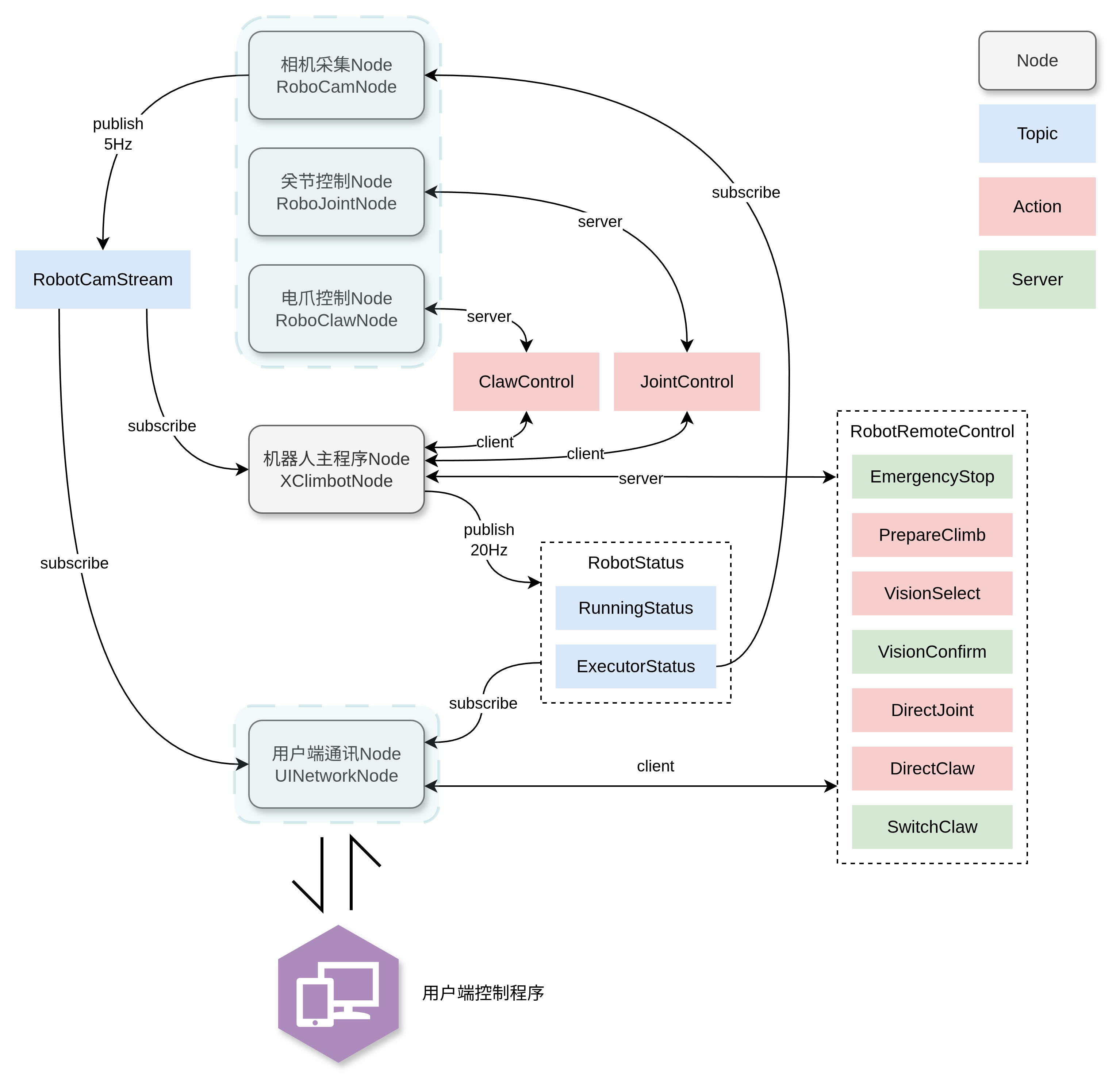
待定,与上塔类似
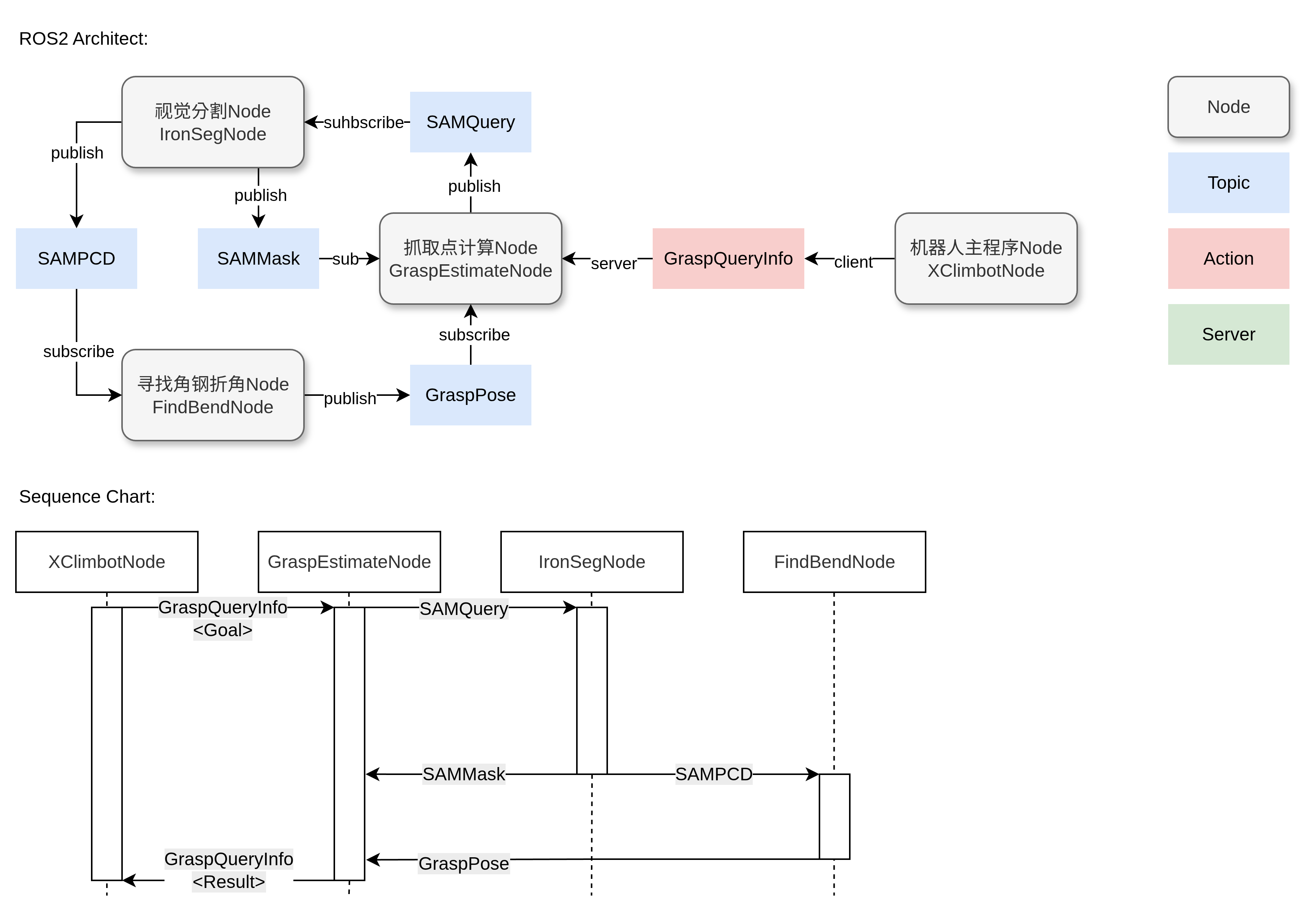
获取3个相机的视频流
作为RobotCamStream 的publisher,发布相 机RGB-D信息(根据订阅的ExecutorStatus中的freeClaw数据来切换相机源)
通过CAN通讯控制机械臂关节
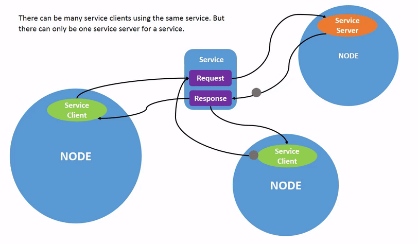
作为JointControl的Action server,响应其他Node的控制指令,响应其他Node的关节状态数据请求
通过485通讯控制机器人电爪
作为ClawControl的Action server,响应主程序Node的控制指令,响应其他Node的电爪状态数据请求
负责机器人的主要运行流程
负责与用户端控制程序进行网络通讯
从主程序Node获取机器人信息,包括机器人运行状态(RobotStatus)和机器人执行器位置(RobotPosition)
获取相机的视频流信息
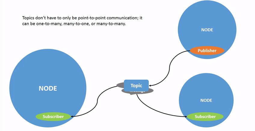
持续publish视频流信息
1 | int8 maincam # 1 for camera_1, 2 for camera_2 |
返回当前机器人的执行器状态:
1 | int8[2] claw_status = 0~4 // 0 for 电爪运动中,1 for 已抓紧,2 for 已释放, 3 for 电爪掉落,4 for 错误,总共两个电爪的数据 |
返回当前机器人的状态
1 | int16 status = -1~10 // -1代表调试功能,开放所有直接控制功能。其余状态见机器人运行流程的图例 |
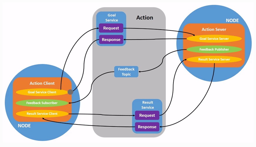
1 | int64[6] goal_angle // each element ∈ [-3600000, 3600000] |
Feedback 为以5Hz频率返回当前关节角度和关节运动状态,表示正在正常执行。
1 | int64[6] current_angle //each element ∈ [-3600000, 3600000] |
Result 用于描述关节运动任务的最终执行结果,仅在任务结束后可获取。
1 | bool success = true | false |
用于控制机器人电爪运动。
1 | // request |
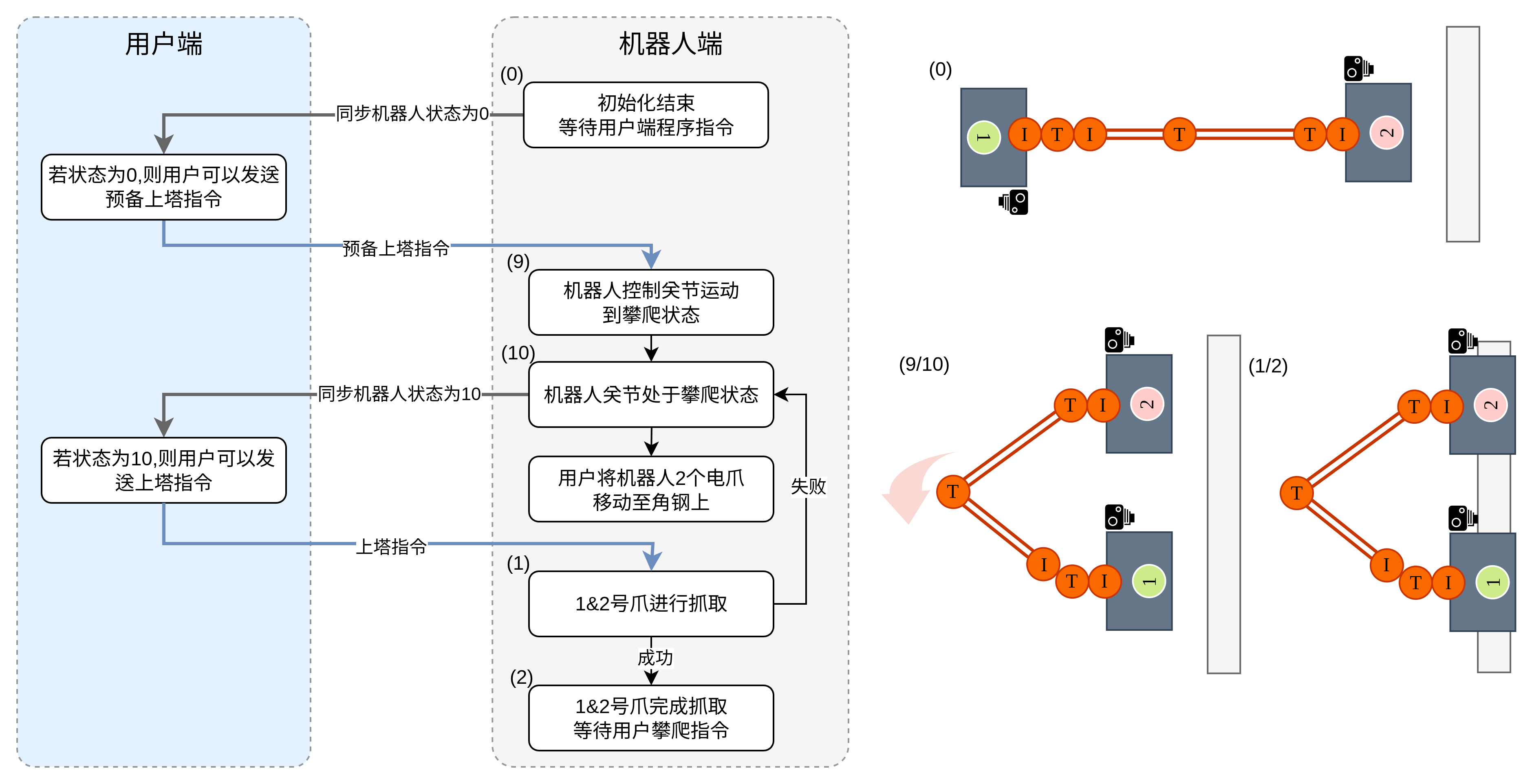
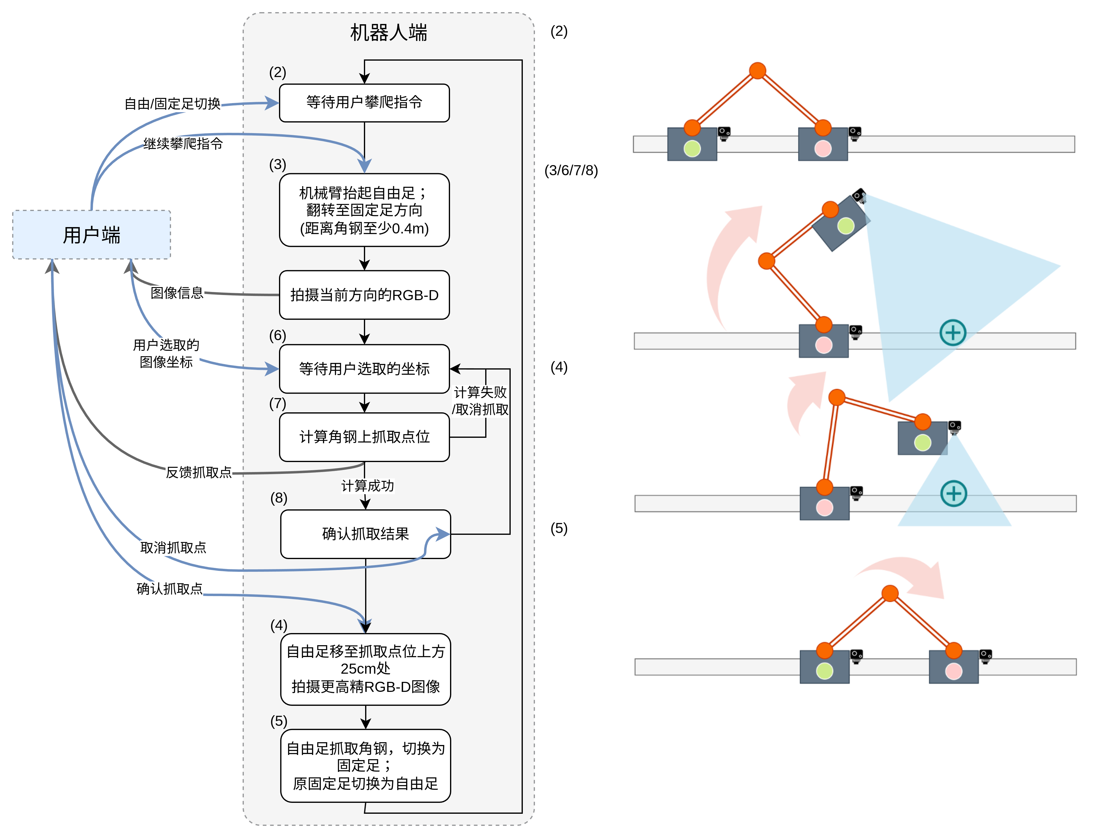
机器人在攀爬结束后两足均抓取于角钢上,此时需要用户发出继续攀爬指令,机器人抬起自由足会运动到拍摄深度图像的位置。
仅当机器人处于status 2(即“等待用户攀爬指令”)时可以发出指令
1 | // request |
用户在用户端点选角钢的坐标数据通过网络发送到用户端通讯Node之后,该Node将坐标信息作为指令目标传给主程序Node,由主程序Node进行图像分析得到抓取点,将mask和抓取点反馈给通讯端Node用于显示。
在用户端程序的视频图像上覆盖显示(半透明)对应的Mask,以及预计抓取点的位置。
这个视觉选择的请求只有当机器人处于status 6 (即“等待用户选取的坐标”)时才有效
1 | //request |
直接控制应该为用户端的一个独立窗口(通过菜单栏选项调出)
用户端通讯Node发给主程序Node的指令,可让用户端直接控制关节的运动。
1 | //request |
直接控制应该为用户端的一个独立窗口(通过菜单栏选项调出)
用户端通讯Node发给主程序Node的指令,可让用户端直接控制电爪的运动。
1 | // request |
1 | //request |
用户端确认抓取点和mask有效与否,将确认信息发回给机器人的用户端通讯Node,用户端通讯Node将确认信息通过service告知主程序Node
这个确认的请求只有当机器人处于status 8 (即“确认抓取结果”)时才有效
1 | //request |
用户端点击切换电爪的按钮后,将切换指令发给机器人的用户通讯端Node,用户端通讯Node将确认信息通过service告知主程序Node
仅当机器人处于status 2时可以切换。
1 | //request |
使用一个package robot_interfaces 用于存放所有的接口定义
例如:
1 | my_robot_interfaces/ |
主程序的核心功能由毕老师实验室团队负责实现。杨总团队需基于主程序框架,在主程序中自行完成本文档所定义的各类 ROS 接口(包括 Action、Service、Topic)的 Server 端实现。
同时,杨总团队需提供与上述接口一一对应的功能测试代码或示例调用代码,以便直接集成或粘贴至主程序中,用于接口联调与功能验证,确保接口定义与实际行为的一致性和可测试性。
典型的主程序python示例为(并非具体实现):
1 | import rclpy |
测试仅针对接口本身,不涉及对于具体机器人运行逻辑的测试。

通过本实验,学习:
使用 二维数组表示离散网格世界
理解并实现 生命游戏的局部规则 → 全局演化
使用 Pygame 进行基础的二维图形显示
使用 键盘事件控制程序行为
将一个问题分解为:
数据结构 → 规则函数 → 显示函数 → 主循环
生命游戏是一个离散、确定性、无随机的元胞自动机:
空间:二维网格
时间:离散时间步
每个格子(细胞)只有两种状态:
活 (1)
死 (0)
对每个细胞,统计它周围 8 个邻居 中活细胞的数量:
| 当前状态 | 活邻居数 | 下一状态 |
|---|---|---|
| 活 | 2 或 3 | 活 |
| 活 | 其他 | 死 |
| 死 | 3 | 活 |
| 死 | 其他 | 死 |
重要思想:
全局复杂行为来自简单的局部规则
在开始写代码前,先规划模块结构:
1 | 生命游戏程序 |
1 | pip install pygame |
1 | import pygame |
1 | CELL_SIZE = 10 # 每个细胞在屏幕上的像素大小 |
解释:
我们的“世界”是逻辑网格
Pygame 显示的是像素
一个细胞 ↔ 一个矩形
1 | ALIVE = 1 |
1 | grid[y][x] |
y:第几行
x:第几列
值:0 或 1
1 | def random_grid(): |
更优雅的写法:
1 | def random_grid(): |
教学要点:
外层列表 → 行
内层列表 → 列
每个位置随机赋值
每个细胞有 8 个邻居:
1 | (-1,-1) (0,-1) (1,-1) |
1 | def count_neighbors(grid, x, y): |
逐行解释:
两层循环遍历 3×3 区域
排除自身
检查是否越界
累加存活细胞数
当前状态 → 决定下一状态
如果边算边改,会影响后续计算
解决方案:
使用一个新的二维数组
1 | def next_generation(grid): |
教学重点:
规则直接翻译成代码
清晰的 if / else 逻辑
新旧网格分离
一个细胞 → 一个矩形
坐标换算:
1 | 屏幕 x = 网格列 * CELL_SIZE |
1 | def draw_grid(screen, grid): |
1 | for x in range(GRID_WIDTH): |
1 | pygame.init() |
1 | grid = random_grid() |
教学重点:
SPACE:推进一代
R:重新初始化
ESC:退出
二维数组 = 世界状态
局部规则 → 全局演化
显示逻辑与计算逻辑分离
主循环 = 事件 + 更新 + 绘制
完整程序:
1 | import pygame |