Math6003 Hw5
Homework 5 Report
Zhichen Tang
124370910020
Exercise 1
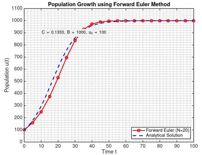
In this first part, I looked at the logistic model for population growth. The main goal was to solve the equation $u’(t) = C u(t) (1 - u(t)/B)$ using a couple of different numerical methods. The parameters were set to $u_0=100$, $B=1000$, and $C=2/15$.
a)
I take the current value and add the slope at that point multiplied by the time step to get the next value.
1 | % Completed feuler.m |
% Completed heun.m
function [t, u, dt] = heun( f, I, u0, N )
dt = (I(2)-I(1))/N;
t = linspace(I(1),I(2),N+1);
u = zeros(1,N+1);
u(1) = u0;
for n = 1:N
u_predictor = u(n) + dt * f(t(n), u(n));
u(n+1) = u(n) + (dt/2) * ( f(t(n), u(n)) + f(t(n+1), u_predictor) );
end
end
<div class="post-content"><img src="/2025/07/14/[OBS]课程-Math6003 Hw5/ex1b.png" alt="" title=""></div>
### c)

After implementing the methods, I ran them with a coarse time step (Deltat=5, corresponding to N=20) and plotted them against the exact solution.

It's pretty clear from the graph that the Heun method does a much better job. Its curve hugs the exact solution line much more tightly than the Forward Euler curve does. This makes sense because it's a higher-order method, so you'd expect it to be more accurate for the same step size.

<div class="post-content"><img src="/2025/07/14/[OBS]课程-Math6003 Hw5/ex1c.png" alt="" title=""></div>

### d)

Next, I repeated the comparison but with a much smaller time step (Deltat=0.05, or N=2000).


Absolutely. With the smaller time step, both methods improved dramatically. The plot shows that the lines for the Euler method, Heun's method, and the exact solution are basically right on top of each other. This really shows how decreasing the step size can significantly reduce the error in numerical solutions. However, the Heun method's absolute error is still lower than the Euler method.

<div class="post-content"><img src="/2025/07/14/[OBS]课程-Math6003 Hw5/ex1d.png" alt="" title=""></div>

---

## Exercise 2

### a)

To solve this, I first had to convert the single 2nd-order equation into a system of two 1st-order equations. I defined a new variable, V(t)=U′(t). This gives the first equation of the system.

Then, I rearranged the original RLC equation to isolate U′′(t):

$$ U''(t) = -\frac{R}{L}U'(t) - \frac{1}{LC}U(t) + \frac{f}{LC} $$

By substituting V for U′ and V′ for U′′, I got the second equation. This allowed me to write the whole system in matrix form, X′=AX+b:

$$\begin{pmatrix} V' \\ U' \end{pmatrix} = \begin{pmatrix} -R/L & -1/(LC) \\ 1 & 0 \end{pmatrix} \begin{pmatrix} V \\ U \end{pmatrix} + \begin{pmatrix} f/(LC) \\ 0 \end{pmatrix} $$
### b)
Stability Analysis of Forward Euler The Forward Euler method is only stable if $|1 + \Delta t \lambda_i| \le 1$ for all eigenvalues ($\lambda_i$) of the matrix A. Using the given component values (L=0.01, C=10, R=0.1), the matrix A becomes: $$ A = \begin{pmatrix} -10 & -10 \\ 1 & 0 \end{pmatrix} $$ I calculated the eigenvalues to be $\lambda = -5 \pm \sqrt{15}$. To ensure stability, the time step $\Delta t$ has to be less than a critical value determined by the eigenvalue with the largest magnitude. The calculation showed that the method is stable only if: $$ \Delta t \le \frac{2}{5 + \sqrt{15}} \approx 0.2254 \text{ s} $$
### c)
Simulating with Forward Euler I ran simulations for three different time steps. The results were a perfect illustration of the stability condition.
<div class="post-content"><img src="/2025/07/14/[OBS]课程-Math6003 Hw5/ex2c.png" alt="" title=""></div>
As you can see: - With **N=43** ($\Delta t \approx 0.233$), the time step was too large, and the solution completely blew up. - With **N=46** ($\Delta t \approx 0.217$), the time step was just inside the stable range, and the solution correctly showed a damped wave. - With **N=500** ($\Delta t = 0.02$), the solution was also stable and much smoother.
### d)
Simulating with Backward Euler Finally, I repeated the same simulations using the Backward Euler method.
<div class="post-content"><img src="/2025/07/14/[OBS]课程-Math6003 Hw5/ex2d.png" alt="" title=""></div>
The difference is night and day. The Backward Euler method was **stable for all three time steps**, even the large one that made the Forward Euler method fail. This shows that implicit methods like Backward Euler are much more robust for systems like this, as they don't have the same strict stability requirements on the time step. While the accuracy still gets better with smaller steps, you can trust it to give a stable answer no matter what.