3D-Scene
Atlas
CLIP
CV
Chemistry
Contrastive-Learning
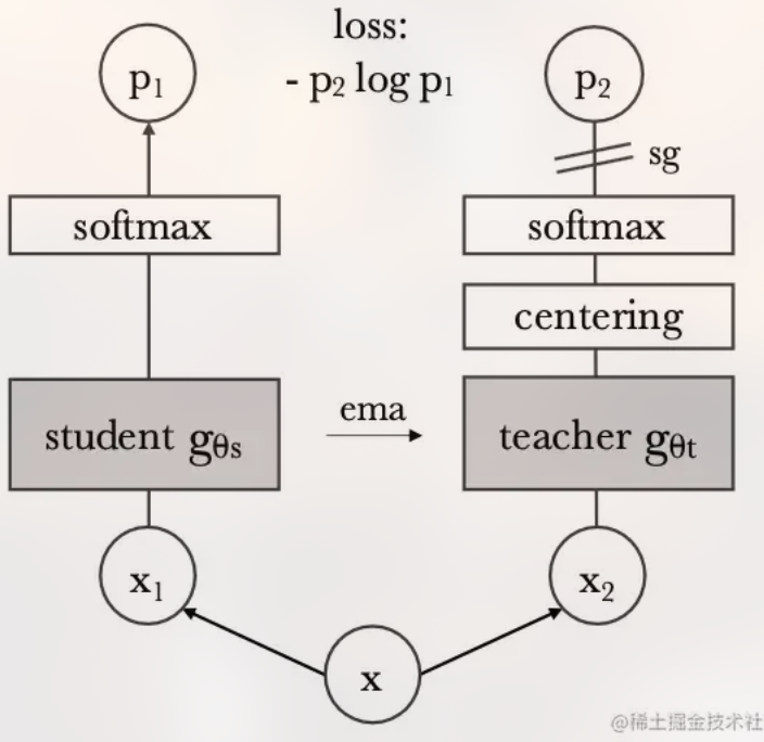
DINO
DT
Diffusion
DiffusionModel
Embodied-AI
FL
FPN
FoundationModel
Gated-NN
HRI
Hierarchical
HumanoidRobot
Image-Grounding
Image-Text
Image-generation
Image2Text
ImgGen
ImitationLearning
LLM
LatentAction
ML
MoE
MoT
MotionGeneration
MR/AR
Message-Passing
Multi-modal
Multi-view
MultiModal
NLP
NN
Object-Detection
Open-Vocabulary
Panoptic
Physical-Scene
PoseEstimation
QML
Quantum
RL
RNN
Real2Sim
Reconstruct
Representation-Learning
RobotLearning
Robotics
Scalability
Scene-graph
Scene-synthesis
Segmentation
Semantic
Sim2Real
Subgraph
Survey
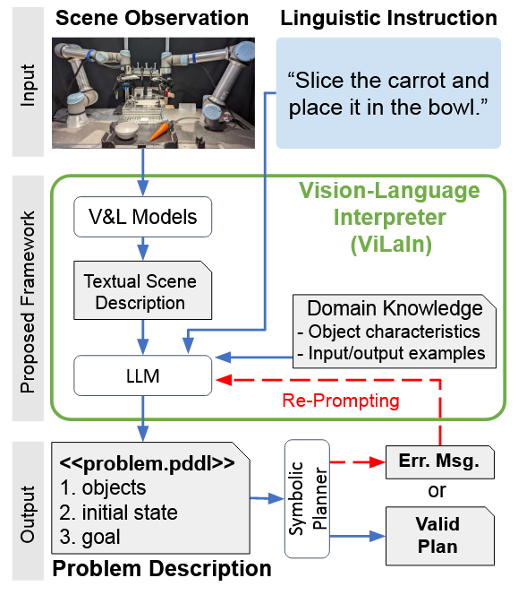
Task-Planning
Transformer
Translation-Embedding
VAE
VLA
VLM
VLP
VQ-VAE
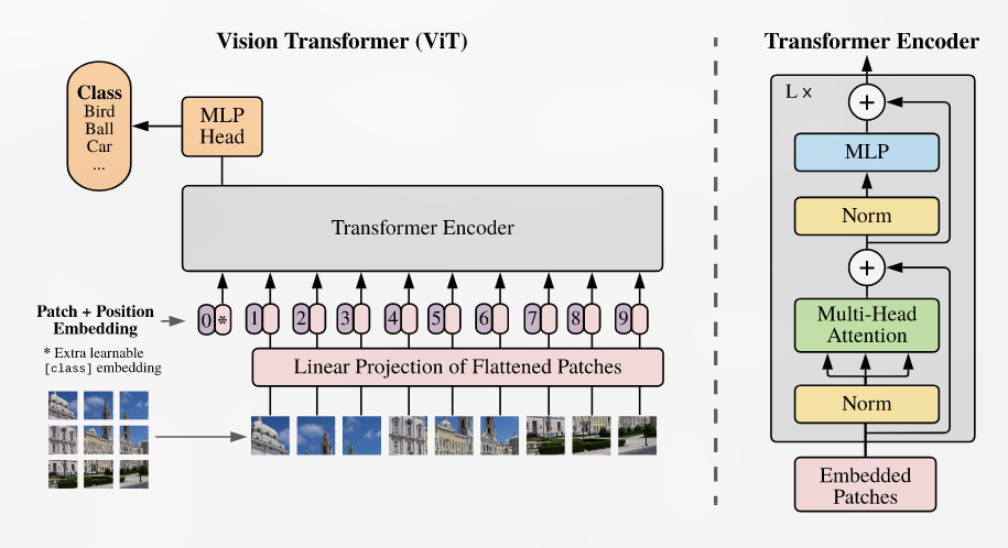
ViT
Visual-Relation
WorldModel
Unified-Multimodal

(Mindmap) Part-level Scene Understanding for Robots
 Part-level Scene Understanding for Robots/Pasted_image_20250414142333.png)
A scene graph is a structural representation, which can capture detailed semantics by explicitly Modeling:
 Contextual Translation Embedding for Visual Relationship Detection and Scene Graph Generation/Pasted_image_20250318160643.png)