
Exercise 1
(a) Polynomial Interpolation
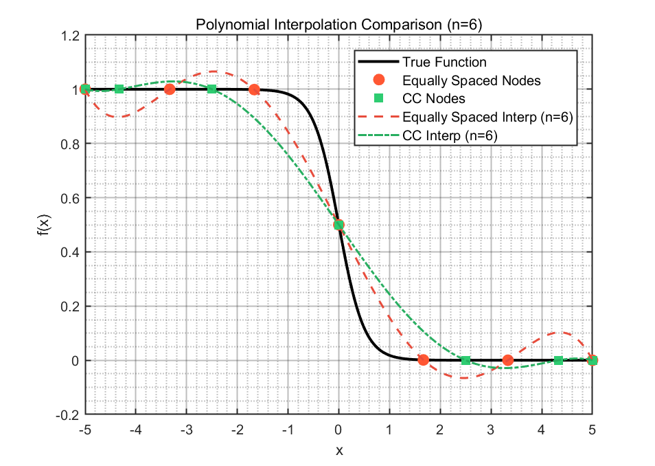
To approximate the function $$f(x) = \frac{1}{1 + \exp(4x)} $$on the interval [-5, 5], polynomial interpolation was performed using polynomials of degree n=6 and n=14. Two types of nodes were considered: equally spaced nodes and Clenshaw-Curtis nodes, the latter computed using the formula
$$
x_i = \frac{a + b}{2} - \frac{b - a}{2} \cos\left(\pi \frac{i}{n}\right), \quad i = 0, \dots, n.
$$
Using polyfit
, the interpolation polynomials were computed based on the function values at the chosen nodes. The polynomials were evaluated using polyval
on a fine grid over [-5, 5] and plotted alongside the true function f(x). The results showed that interpolation with Clenshaw-Curtis nodes provided better approximation near the boundaries, especially for n=14, reducing the Runge phenomenon that is prominent with equally spaced nodes.
(b) Piecewise Linear Interpolation
For the same values of n=6 and n=14, piecewise linear interpolation was carried out using interp1
with equally spaced nodes. The linear interpolant $$p_{1,h}$$ was constructed over n subintervals of length $$h = \frac{10}{n}$$. The resulting piecewise linear functions were evaluated on a fine grid and compared graphically with the original function f(x). While less smooth than the high-degree polynomials, the linear interpolation captured the overall trend of the function and showed more stable behavior near the interval edges.
(c) Error Analysis
To quantitatively assess the interpolation accuracy, the maximum approximation error
$$
E_n = \max_{x \in [-5, 5]} |f(x) - p_n(x)|
$$
was computed for n=2 to 40 for both equally spaced and Clenshaw-Curtis nodes. Similarly, the maximum error for piecewise linear interpolation, $$E_{1,h}$$, was evaluated for the same range of n. A loop was used to iterate over n, computing and storing the errors. The results were visualized on a log-scale plot with respect to n. The plots clearly demonstrated that Clenshaw-Curtis interpolation achieves significantly better accuracy with increasing n, while equally spaced nodes lead to instability and large errors as n grows. Piecewise linear interpolation, although low-order, exhibited stable and predictable convergence.
Exercise 2
(a) Equally Distributed Nodes
The function $f(x) = \sin(x) + x$ was interpolated on the interval [0,10] using Lagrange polynomial interpolation. Two degrees were considered: $n = 4$ and $n = 15$, corresponding to $n + 1$ equally spaced nodes. For each value of n, two datasets were created: one using the exact function values $y_i = f(x_i)$, and the other using perturbed values $z_i = y_i + \epsilon_i$, where $\epsilon_i \sim \text{Uniform}(-0.1, 0.1)$. Using polyfit
and polyval
, the interpolation polynomials were computed and evaluated on a dense grid for visualization.
The results show that for n = 4, both the unperturbed and perturbed interpolants approximate the true function reasonably well, though the perturbed one deviates slightly. For n = 15, the interpolant using exact values exhibits oscillatory behavior near the boundaries, a clear manifestation of the Runge phenomenon. The polynomial interpolant using noisy data becomes highly unstable, demonstrating extreme sensitivity to small perturbations in the input values.
(b) Clenshaw-Curtis Nodes
The same procedure was repeated using Clenshaw-Curtis nodes computed using the cosine-based formula. For both n = 4 and n = 15, interpolation polynomials were fitted using the exact and perturbed data values. When visualized, the interpolants using Clenshaw-Curtis nodes performed significantly better near the boundaries compared to those using equally spaced nodes. Particularly for n = 15, the polynomial interpolant with exact values closely follows the true function, with reduced oscillations. Even when perturbations are introduced, the polynomial remains relatively stable and does not exhibit the extreme sensitivity observed in the equally spaced case. This confirms that Clenshaw-Curtis nodes enhance numerical stability in high-degree interpolation.
(c) Piecewise Linear Interpolation
Piecewise linear interpolation was implemented using interp1
on equally spaced nodes for both n = 4 and n = 15. As before, both the exact and perturbed datasets were used to construct the interpolants. The linear interpolants followed the general shape of the original function and remained visually close to the true curve even when noise was added. This behavior was consistent across both values of n. While less accurate than high-degree polynomial interpolation in smooth regions, the piecewise linear approach showed strong robustness to noise and did not exhibit oscillations or instability, making it a reliable method for interpolating noisy data.
Exercise 3
(a) Least Squares Polynomial of Degree 4
The file data1.mat
was loaded to obtain the dataset $(x_i, y_i)$, where $y_i = \sin(x_i) + x_i + \epsilon_i$, and $epsilon_i$ represents Gaussian noise with zero mean and standard deviation $σ=0.1$. A degree-4 least squares polynomial $p^{LS}_4$ was fitted using polyfit(x, y, 4)
. On the same plot, the original function $f(x) = \sin(x) + x$, the noisy data points $(x_i, y_i)$, and the polynomial $p^{LS}_4(x)$ were displayed. The polynomial provided a smooth approximation that followed the general trend of the function, mitigating the effect of noise.
(b) Higher-Degree Least Squares Polynomials (m = 7, 15)
The procedure was repeated for polynomial degrees $m = 7$ and $m = 15$. For $m = 7$, the approximation improved slightly, with the polynomial capturing more curvature of the underlying function. However, at $m = 15$, overfitting became evident—the polynomial began to follow the noise, especially near the edges of the interval. This illustrates the typical variance-bias tradeoff in polynomial regression: higher degrees reduce bias but increase sensitivity to noise.
(c) Approximation Error vs. Degree
To assess the accuracy of the least squares fit, the error $E(p^{LS}m, f) = \max{x \in [0, 10]} |f(x) - p^{LS}_m(x)|$
was computed for degrees m = 1 to 1515, evaluated over a fine grid. The error was then plotted as a function of m on a semi-logarithmic scale. The plot showed a decreasing trend in the error for small m, reaching a minimum at some intermediate degree. Beyond that, the error increased, reflecting overfitting. This confirms that, for noisy data, the optimal degree is not necessarily high.
(d) Noise Variance Estimation and Error Comparison
The variance of the noise was estimated using the formula
$\hat{\sigma}^2 = \frac{1}{n - m} \sum_{i=1}^{n+1} \left( y_i - p^{LS}_m(x_i) \right)^2,$
with m = 4 and n + 1 = 20. The estimated variance $\hat{\sigma}$ was then used to compute the expected approximation error scale
$\hat{\sigma} \cdot \sqrt{\frac{m + 1}{n + 1}}.$
The previously observed minimal error matched this estimate in magnitude, validating the analytical approximation. A comparison with the theoretical value $\sigma \cdot \sqrt{(m+1)/(n+1)}$ was also performed, showing good agreement.
(e) Large-Scale Data: n + 1 = 20000
The analysis from parts (a) to (d) was repeated using the dataset in data2.mat
, which contains n + 1 = 20000 samples. The results demonstrated a dramatic improvement in the stability and accuracy of least squares fitting. Overfitting effects were less pronounced even at higher polynomial degrees due to the large number of samples. The error curve in (c) showed a more gradual and consistent decrease, and the noise influence was better averaged out. Variance: 0.04814, Bound ≈ 0.00347
(f) Error Comparison Between Small and Large Datasets
The minimal approximation error achieved using the larger dataset was significantly smaller than that obtained from the 20-point dataset. This reflects the benefit of larger sample sizes in reducing noise impact and improving model robustness. Moreover, the estimated noise error scale $\hat{\sigma} \cdot \sqrt{(m+1)/(n+1)}$ decreased accordingly due to the much larger denominator, reinforcing the statistical intuition.
Exercise 4
the Lagrange interpolation error at any point x in the interval containing the nodes is given by
$f(x) - p_n(x) = \frac{f^{(n+1)}(\xi)}{(n+1)!} \prod_{k=0}^n (x - x_k)$
Taking the absolute value yields the error bound
$|f(x) - p_n(x)| \leq \frac{M}{(n+1)!} \left| \prod_{k=0}^n (x - x_k) \right|$
where $p_n(x)$ is the interpolating polynomial of degree n through n+1 points. For both functions, the interpolation degree was set to n=4, which requires the fifth derivative of the target function.
For the function $f_1(x) = \cosh(x)$, the interpolation nodes were defined as $x_k = -1 + \frac{k}{2}$for $k = 0, 1, \dots$, giving equally spaced points in the interval [−1,1]. The fifth derivative of $\cosh(x)$ is $\sinh(x)$, since derivatives of hyperbolic functions follow a repeating pattern. The maximum of $|\sinh(x)|$ over[−1,1] occurs at x = 1, where $\sinh(1) \approx 1.175$. Substituting into the error formula, the upper bound depends on this derivative value and the absolute value of the product of linear terms $(x - x_k),$ divided by $5! = 120$.
For the function $f_2(x) = \cos(x) + \sin(x)$, the interpolation nodes were chosen as $x_k = -\frac{\pi}{2} + \frac{\pi k}{4}$ for $k = 0, \dots, 4$, covering the interval [−2π,2π]. The fifth derivative of $f_2$ is $-\cos(x) + \sin(x)$, based on the periodic differentiation cycle of sine and cosine. The maximum of the absolute value of this expression was found numerically over the interpolation interval. This value was then used in the same error formula as above, with the factorial and the product of distances from the interpolation nodes.
In both cases, the error bound reflects how the function’s higher-order smoothness and the choice of interpolation nodes influence the potential deviation between the true function and its polynomial approximation. The approach confirms that even for smooth functions, the interpolation error can grow significantly away from the nodes if the derivatives are large or if the node distribution leads to large oscillations in the interpolating polynomial.